论文绘图时经常需要多图嵌套，正好最近绘图用到了，记录一下使用Python实现多图嵌套的过程。

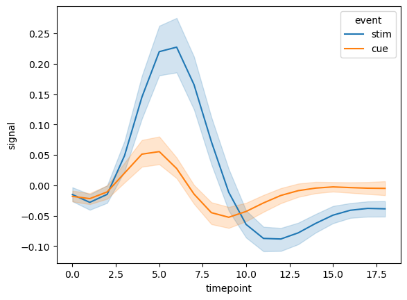
首先，实现 Seaborn 分别绘制折线图和柱状图。

	'''绘制折线图'''
	import seaborn as sns
	import matplotlib.pyplot as plt
	import warnings
	warnings.filterwarnings("ignore", "use_inf_as_na")
	# 获取绘图数据
	df_fmri=sns.load_dataset("fmri")
	# 绘制折线图
	sns.lineplot(data=df_fmri, x="timepoint", y="signal", hue="event")
	# 创建绘图数据
	df_bar=df_fmri[['subject','signal']].groupby('subject',observed=True).agg('max').reset_index()
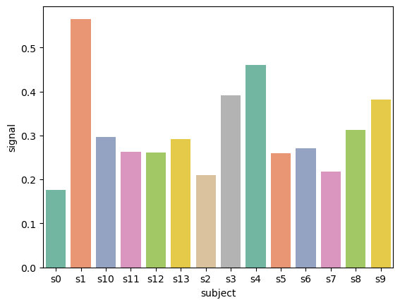
	# 绘制条形图
	ax_bar=sns.barplot(
	data=df_bar,
	x="subject", y="signal",
	palette='Set2',
	)

接下来实现条形图与折线图的嵌套，核心是使用 inset_axes 函数创建一个新的轴，然后再绘制第二个图时指定绘图的轴为刚才新建的轴。

	from mpl_toolkits.axes_grid1.inset_locator import inset_axes
	import matplotlib.pyplot as plt
	# 获取绘图数据
	df_fmri = sns.load_dataset("fmri")
	df_bar=df_fmri[['subject','signal']].groupby('subject',observed=True).agg('max').reset_index()
	# 绘制折线图
	ax=sns.lineplot(data=df_fmri, x="timepoint", y="signal", hue="event")
	plt.legend(loc='upper left')
	# 使用 inset_axes 函数添加一个轴，用来显示条形图
	ax_bar = inset_axes(
	ax, # 父轴
	width='40%', height='50%', # 新轴相对于父轴的长宽比例
	loc='lower left', # 新轴的锚点相对于父轴的位置
	bbox_to_anchor=(0.55,0.45,1,1), # 新轴的bbox
	bbox_transform=ax.transAxes # bbox_to_anchor 的坐标基准
	)
	# 绘制条形图
	ax_bar=sns.barplot(
	data=df_bar,
	x="subject", y="signal",
	palette='Set2',
	ax=ax_bar
	)

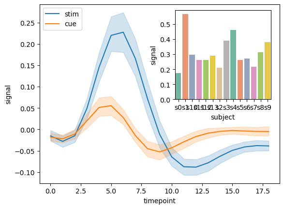
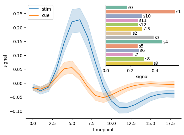
可以看到，右上角的条形图显得很拥挤，x轴标注相互重叠比较严重，因此，考虑将条形图由纵向变为横向，在 Seaborn 绘图时交换 x 轴和 y 轴就能实现。此外，bar上方的空间也比较大，考虑将x轴的标注标注到bar上方，以进一步节约空间。bar的标注可以通过 ax.bar_label() 函数实现，该函数不仅可以直接标注每个bar的数值，也可以自定义要标注的内容和格式。修改后的代码和结果图如下：

	from mpl_toolkits.axes_grid1.inset_locator import inset_axes
	import matplotlib.pyplot as plt
	# 准备数据
	df_fmri = sns.load_dataset("fmri")
	df_bar=df_fmri[['subject','signal']].groupby('subject',observed=True).agg('max').reset_index()
	# 绘制折线图
	ax=sns.lineplot(data=df_fmri, x="timepoint", y="signal", hue="event")
	plt.legend(loc='upper left')
	# 使用 inset_axes 函数添加一个轴，用来显示条形图
	ax_bar = inset_axes(
	ax, # 父轴
	width='47%', height='52%', # 新轴相对于父轴的长宽比例
	loc='lower left', # 新轴的锚点相对于父轴的位置
	bbox_to_anchor=(0.5,0.44,1,1), # 新轴的bbox
	bbox_transform=ax.transAxes # bbox_to_anchor 的坐标基准
	)
	# 绘制条形图
	ax_bar=sns.barplot(
	data=df_bar,
	# 交换 x 轴和 y 轴列名实现横向条形图
	x="signal", y="subject",
	palette='Set2',
	ax=ax_bar
	)
	# 使用 sns 的 bar_label 函数为条形图添加标注
	ax_bar.bar_label(
	ax_bar.containers[0], # 条形图的 BarContainer 对象
	labels=df_bar['subject'], # 要标注的labels，默认为 bar 的数值，此处传入自定义的label序列
	label_type='edge', # 标注显示的位置，可选 edge 或 center
	padding=2, # 标注与bar之间的距离
	# fmt='%.2f' # 标注格式化字符串
	fontsize=10 # 设置标注的字体大小
	)
	# 为了避免标注超出绘图范围，将x轴的绘图范围扩大
	plt.xlim(0,0.62)
	# 隐藏左侧y轴
	ax_bar.yaxis.set_visible(False)
	# 去除多余的轴线
	sns.despine()